ベンチで「効果を見つけた」と思ったら、測定のぶれだった I Thought My Benchmark Found an Effect, but It Was Measurement Noise
はじめに
第2回で、KV キャッシュの量子化を 使わないと決めました。理由はこう書いています。
q8_0 は f16 と同等の perplexity を示し品質劣化はほぼ無い。 しかし f16 が収まる環境では f16 のほうが速い。毎トークン逆量子化が走るため。
この判断には弱点がありました。根拠が他所の計測だったことです。 「64K 深度で f16 比 55% まで落ちる」という報告を読んで、 自分の環境では測らずに不採用にしていました。
その後コンテキストを 16K から 64K に広げたので、前提を確かめる必要が出てきました。 測りました。そして一度、間違った結論を出しました。その記録です。
何を測るか
llama-bench には -d(n-depth)があります。
KV キャッシュに指定トークン数を積んだ状態から生成を始めるので、
「会話が長くなったとき、生成がどれだけ遅くなるか」を直接測れます。
llama-bench -hf <model> -ngl 99 -fa 1 -b 8192
            -p 0 -n 128 -d 0,4096,16384,32768
-p 0 でプロンプト処理を外し、生成だけを切り出します。
まず f16 で測り、次に -ctk q8_0 -ctv q8_0 で同じことをやりました。
1 回目: 判断が覆った(と思った)
| 深度 | f16 | q8_0 | 差 |
|---|---|---|---|
| 0 | 16.79 | 18.36 | +9.4% |
| 4,096 | 16.27 | 18.17 | +11.7% |
| 16,384 | 15.05 | 16.54 | +9.9% |
| 32,768 | 14.29 | 15.38 | +7.6% |
全深度で q8_0 が速い。 しかもばらつきも小さい。
このとき、説明まで思いついていました。
この機体は一貫して帯域律速だった。密 27B より MoE が 5.7 倍速いのも、
-bは効くが-ubは効かないのも、全部帯域で説明がついた。 KV を量子化すれば読み出しが減る。帯域律速の環境では q8_0 が有利なのではないか。
筋が通って聞こえます。第2回が参照した報告はおそらく dGPU のもので、 そちらは演算律速だから逆量子化のコストがそのまま損になる。 こちらは帯域律速だから得をする——。
もっともらしい説明ほど危ない、という話をこれから書きます。
引っかかった点
表を眺めていて、深度 0 で 9.4% の差がついているのが気になりました。
深度 0 は KV キャッシュが空です。空のキャッシュを量子化しても、 読むものが無いのだから速度は変わらないはずです。
帯域律速の仮説が正しいなら、差は深いところほど大きくなるべきで、 深度 0 ではゼロに近いはずでした。実際の表は逆で、 深度 0 がいちばん差が大きく、深くなるほど縮んでいます。
説明と観測が合っていません。
2 回目: 測り直した
llama-bench は条件をカンマ区切りで受け取れます。
1 回の起動の中で f16 と q8_0 を交互に、各 5 回ずつ測りました。
llama-bench ... -d 0,32768 -ctk f16,q8_0 -ctv f16,q8_0 -r 5結果が逆になりました。
| type_k | type_v | 深度 0 | 深度 32,768 |
|---|---|---|---|
| f16 | f16 | 18.57 ± 0.51 | 15.65 ± 0.23 |
| f16 | q8_0 | 17.60 ± 0.99 | 14.14 ± 0.41 |
| q8_0 | f16 | 17.58 ± 0.35 | 15.10 ± 0.35 |
| q8_0 | q8_0 | 17.71 ± 1.03 | 14.06 ± 0.37 |
f16 が最速です。 深度 32K で q8_0 比 +11.3%(15.65 対 14.06)、 誤差範囲も重なっていません。
そして深度 0 では、差が消えました。 18.57 ± 0.51 と 17.71 ± 1.03 は範囲が重なります。 KV が空なら量子化は効かない、という物理どおりです。
第2回の判断は正しかったわけです。
何が起きていたのか
1 回目と 2 回目で、同じ f16 / 深度 0 の値が違います。
1 本目: 16.79
3 本目: 18.57   ← 同じ設定なのに +10.6%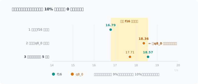
実行間のばらつきが約 10% ありました。 測ろうとしていた差(約 9%)が、そっくりその中に埋もれていたわけです。
1 本目と 2 本目は別プロセスで、順番に走らせました。 その間にウォームアップの状態も、電力もサーマルも変わります。 2 本目が有利な条件で走っただけでした。
「q8_0 のほうが速い」という観測は、条件の差ではなく順番の差を見ていたことになります。
帯域律速の仮説も外れていた
ついでに、私が立てた説明も間違っていました。
KV を量子化すれば読み出しは確かに減ります。 しかし逆量子化のコストのほうが上回っていました。帯域律速の環境でも、です。
細かい発見として、V を量子化するほうが K より損でした。
| 深度 32,768 | |
|---|---|
| K も V も f16 | 15.65 |
| K だけ q8_0 | 15.10 |
| V だけ q8_0 | 14.14 |
| K も V も q8_0 | 14.06 |
K だけなら劣化 3.5%、V だけだと 9.7%。 q8_0 にするなら K から、というのは覚えておく価値がありそうです。
収穫: 深度による劣化は緩やかだった
誤りは誤りとして、新しく分かったこともあります。
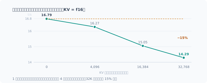
| 深度 | tg128 | 深度 0 比 |
|---|---|---|
| 0 | 16.79 | — |
| 4,096 | 16.27 | −3% |
| 16,384 | 15.05 | −10% |
| 32,768 | 14.29 | −15% |
32K まで積んでも 15% 減です。 第2回が参照した「64K 深度で f16 比 55%」という報告に比べると、 傾きがかなり緩いことになります。
長い会話やコードレビューで深いコンテキストを使っても、 速度面の心配は小さいと言えます。
この 4 点は 1 回の起動の中で深度だけを振った値なので、互いに比較できます。 さっき批判した測り方をここではしていません。
教訓
差が 10% 前後なら、まず測定系のばらつきを確かめる。
効果の大きさを測る前に、同じ条件を 2 回測ってどれだけ動くかを見るべきでした。 それをやっていれば、1 回目の表を見た瞬間に「この差はノイズの範囲だ」と分かりました。
別々に起動したベンチは比較できない。
llama-bench に限らず、プロセスを分けた時点で
ウォームアップ・電力・サーマル・キャッシュの状態が揃わなくなります。
比較したい条件は、1 回の起動の中で振る。
-ctk f16,q8_0 -ctv f16,q8_0 -r 5説明が思いついたときこそ疑う。
今回いちばん危なかったのは、「帯域律速だから q8_0 が有利」という説明が すぐ出てきてしまったことです。しかもこれまでの観測と整合していました。
もっともらしい説明は、間違った数字に説得力を与えてしまいます。 助かったのは、説明のほうが別の予測(深度 0 では差が出ないはず)を持っていたからでした。 その予測が外れていたので、測り直す気になりました。
説明できたと思ったら、その説明が他に何を予測するかを確かめる。 そこが合っていなければ、説明か数字のどちらかが間違っています。
まとめ
- 過去の判断(KV は f16 のまま)を検証したら、一度は逆の結論が出た
- 深度 0 で差が出るのは物理的におかしいと気づき、測り直したら元の判断が正しかった
- 原因は実行間のばらつき 10%。測ろうとした差がその中に埋もれていた
- 設定は変更なし。深度 32K での劣化は 15% と緩やかという収穫は残った
- q8_0 を使うなら K から。V の量子化のほうが損が大きい
検証して「やっぱり正しかった」で終わる話でしたが、 途中で間違えた過程のほうが、自分には収穫でした。
Introduction
In part 2, I decided not to use KV cache quantization. Here’s the reason I gave:
q8_0 shows perplexity on par with f16, with almost no quality loss. But where f16 fits, f16 is faster, because dequantization runs on every token.
That decision had a weak spot: its basis was someone else’s measurement. I had read a report that “at 64K depth it drops to 55% of f16”, and rejected it without measuring on my own machine.
Since then I had widened the context from 16K to 64K, so I needed to check that assumption. I measured it. And at one point, I reached the wrong conclusion. This is the record of that.
What to Measure
llama-bench has -d (n-depth).
It starts generating with the given number of tokens already in the KV cache,
so you can directly measure “how much slower generation gets as the conversation grows”.
llama-bench -hf <model> -ngl 99 -fa 1 -b 8192
            -p 0 -n 128 -d 0,4096,16384,32768
-p 0 removes prompt processing and isolates generation alone.
I measured with f16 first, then did the same with -ctk q8_0 -ctv q8_0.
Round 1: The Decision Was Overturned (Or So I Thought)
| Depth | f16 | q8_0 | Difference |
|---|---|---|---|
| 0 | 16.79 | 18.36 | +9.4% |
| 4,096 | 16.27 | 18.17 | +11.7% |
| 16,384 | 15.05 | 16.54 | +9.9% |
| 32,768 | 14.29 | 15.38 | +7.6% |
q8_0 was faster at every depth. And with less variance, too.
At that point, I had even come up with an explanation.
This machine has been consistently bandwidth-bound. MoE being 5.7x faster than dense 27B,
-bhelping while-ubdoesn’t: bandwidth explained all of it. Quantizing KV reduces reads. On a bandwidth-bound machine, maybe q8_0 comes out ahead.
It sounds plausible. The report part 2 relied on was probably from a dGPU, which is compute-bound, so the dequantization cost is a straight loss there. Here it’s bandwidth-bound, so it comes out ahead…
What follows is about how the more plausible the explanation, the more dangerous it is.
What Bothered Me
Looking over the table, the 9.4% difference at depth 0 bothered me.
At depth 0, the KV cache is empty. Quantizing an empty cache shouldn’t change the speed, since there’s nothing to read.
If the bandwidth-bound hypothesis were right, the gap should grow at greater depths and be close to zero at depth 0. The actual table was the opposite: the gap was largest at depth 0 and shrank as it got deeper.
The explanation and the observations didn’t match.
Round 2: Measuring Again
llama-bench accepts comma-separated conditions.
Within a single launch, I measured f16 and q8_0 alternately, 5 times each.
llama-bench ... -d 0,32768 -ctk f16,q8_0 -ctv f16,q8_0 -r 5The result flipped.
| type_k | type_v | Depth 0 | Depth 32,768 |
|---|---|---|---|
| f16 | f16 | 18.57 ± 0.51 | 15.65 ± 0.23 |
| f16 | q8_0 | 17.60 ± 0.99 | 14.14 ± 0.41 |
| q8_0 | f16 | 17.58 ± 0.35 | 15.10 ± 0.35 |
| q8_0 | q8_0 | 17.71 ± 1.03 | 14.06 ± 0.37 |
f16 is the fastest. At 32K depth it’s +11.3% over q8_0 (15.65 vs. 14.06), and the error ranges don’t overlap.
And at depth 0, the difference disappeared. The ranges of 18.57 ± 0.51 and 17.71 ± 1.03 overlap. Just as physics says: if the KV cache is empty, quantization has no effect.
The decision in part 2 was right after all.
What Was Going On
Between round 1 and round 2, the value for the same f16 / depth 0 setting differs.
1 本目: 16.79
3 本目: 18.57   ← 同じ設定なのに +10.6%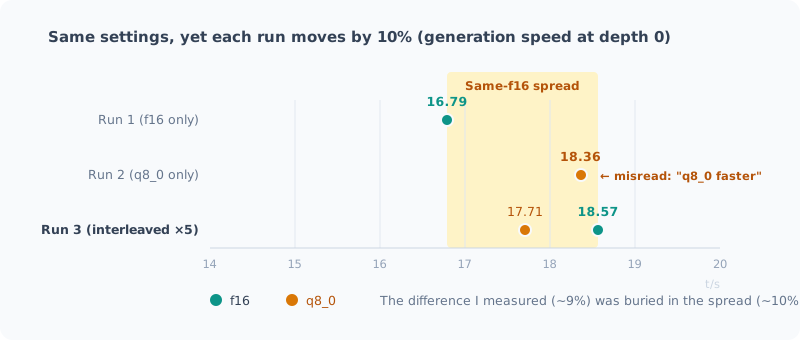
There was about 10% variation between runs. The difference I was trying to measure (about 9%) was buried entirely inside it.
Runs 1 and 2 were separate processes, run one after the other. In between, the warm-up state, power, and thermals all change. Run 2 just happened to run under more favorable conditions.
The observation that “q8_0 is faster” was really showing a difference in order, not in settings.
The Bandwidth-Bound Hypothesis Was Wrong, Too
On top of that, the explanation I came up with was wrong as well.
Quantizing KV does reduce reads. But the dequantization cost outweighed it. Even on a bandwidth-bound machine.
A smaller finding: quantizing V costs more than quantizing K.
| Depth 32,768 | |
|---|---|
| Both K and V f16 | 15.65 |
| K only q8_0 | 15.10 |
| V only q8_0 | 14.14 |
| Both K and V q8_0 | 14.06 |
K alone loses 3.5%; V alone loses 9.7%. If you use q8_0, start with K: that seems worth remembering.
What I Gained: Slowdown with Depth Was Gradual
Mistakes aside, I did learn something new.
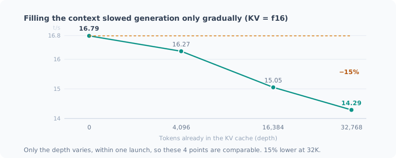
| Depth | tg128 | vs. depth 0 |
|---|---|---|
| 0 | 16.79 | — |
| 4,096 | 16.27 | −3% |
| 16,384 | 15.05 | −10% |
| 32,768 | 14.29 | −15% |
Even with 32K filled, it’s only 15% lower. Compared with the report part 2 relied on, “55% of f16 at 64K depth”, the slope is much gentler.
So even when using deep context for long conversations or code reviews, speed is not much of a concern.
These 4 points are values from a single launch where only the depth varied, so they can be compared with each other. I’m not using the method I just criticized here.
Lessons
When the difference is around 10%, check the measurement noise first.
Before measuring the size of an effect, I should have looked at how much the same setting moves when measured twice. If I had done that, I’d have known the moment I saw the first table that “this difference is within the noise”.
Benchmarks from separate launches can’t be compared.
Not just llama-bench: the moment you split processes,
the warm-up, power, thermal, and cache states no longer line up.
Vary the conditions you want to compare within a single launch.
-ctk f16,q8_0 -ctv f16,q8_0 -r 5Be most suspicious when an explanation comes to mind.
The most dangerous part this time was that the explanation “it’s bandwidth-bound, so q8_0 wins” came to me right away. And it was consistent with my earlier observations.
A plausible explanation lends credibility to wrong numbers. What saved me was that the explanation carried another prediction (there should be no difference at depth 0). That prediction failed, which is what made me measure again.
When you think you’ve explained something, check what else that explanation predicts. If that doesn’t match, either the explanation or the numbers are wrong.
Summary
- When I re-checked a past decision (keep KV at f16), I reached the opposite conclusion at first
- I noticed that a difference at depth 0 was physically odd, measured again, and the original decision was right
- The cause was 10% variation between runs. The difference I was measuring was buried in it
- No settings changed. What I gained was that slowdown at 32K depth is a gentle 15%
- If you use q8_0, start with K. Quantizing V costs more
It was a story that ended with “it was right after all”, but for me, the process of getting it wrong along the way was the bigger takeaway.
関連記事 Related Posts
ローカルLLMのベンチマークの取り方(チェックリスト付き) How to Benchmark a Local LLM (with a Checklist)
ローカルLLMの速度や品質を測るときに、結果を信用できるものにする手順をまとめました。同じ条件でも1割ぶれる、順番で結果が変わる、裏の処理で5倍ぶれる、採点器が壊れている。実際に踏んだ失敗から作った、測る前・測っている間・測ったあとのチェックリストです。 I put together the steps that make the results trustworthy when measuring the speed or quality of a local LLM. The same conditions vary by 10%, the order changes the result, background work causes 5x swings, and the grader is broken. This is a before, during and after checklist built from mistakes I actually made.
コンテキストを 128K まで伸ばしたら、壁はメモリではなく待ち時間だった I Stretched the Context to 128K, and the Wall Was Waiting Time, Not Memory
ローカルLLMのコンテキストを32Kから128Kまで伸ばして測りました。予想していたメモリ不足は起きず、理由はモデルの構造にありました。代わりに見えた壁はプロンプトの取り込み時間で、128Kを読ませるだけで21〜24分かかります。途中で自分の自動起動に計測を汚された話も含みます。 I stretched my local LLM's context from 32K to 128K and measured it. The memory shortage I expected never happened, and the reason lay in the model's architecture. The wall I hit instead was prompt ingestion time: just reading 128K takes 21–24 minutes. It also covers how my own auto-start polluted the measurements along the way.
ローカルLLMを13回測って、測定のほうが19回間違っていた I Measured My Local LLM 13 Times, and the Measurements Were Wrong 19 Times
ローカルLLM環境の構築と検証を13本の記事に書くあいだに、測定する側が間違っていた場面が19回ありました。比べ方、採点器のバグ、外からの割り込み、前提の取り違え、動いていなかった安全装置。気づいたきっかけを数えると、半分以上は「ありえない値」か「生データ」でした。測る前のチェックリストにまとめます。 While writing 13 posts about building and testing my local LLM setup, the measuring side was wrong 19 times: how I compared, bugs in the grader, interruptions from outside, wrong assumptions, and safety mechanisms that weren't working. Counting how I noticed, more than half came from "impossible values" or "raw data". I turn them into a checklist for before measuring.